Gem
An Elastic, Local Similarity Measure with Automatic Trend Adjustment
Welcome to the supplementary webpage for the GEM paper
This page is intended to give additional information and material including all data sets and source code. You can download all supplementary material in a single zip file (see left) or browse the repository at github.
cDTW vs. GEM dendrograms and the Metal dataset
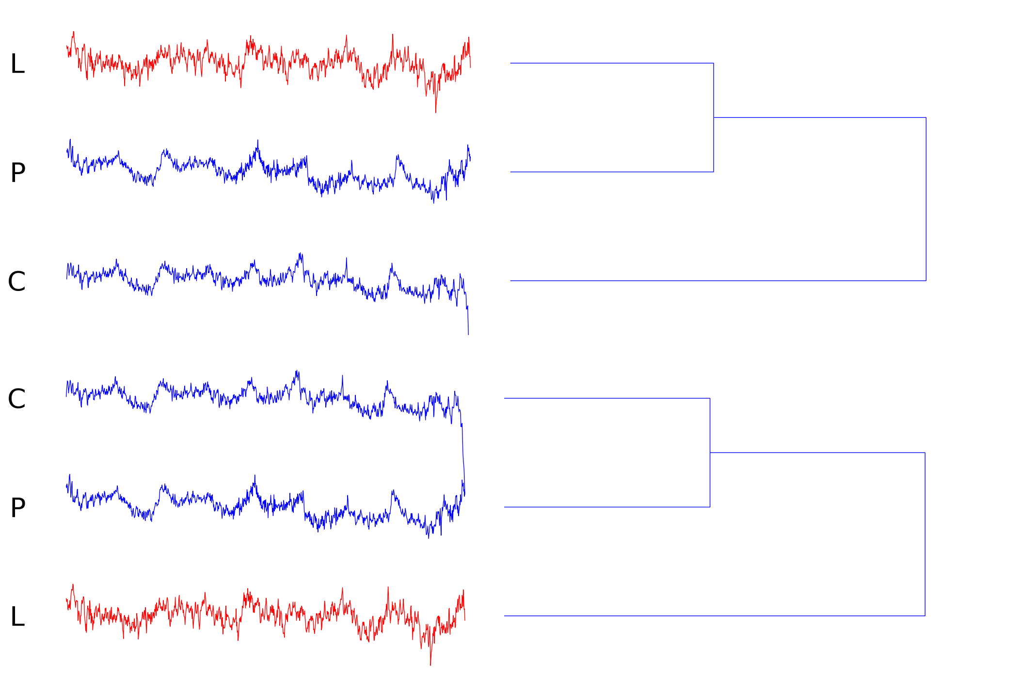
This sections provides additional dendrograms obtained on the left split (indices 100-499) of the metal dataset. We only state three examples of different types for brevity. All misclassifications of cDTW on this split can be found here in pdf or png format. For a given index the upper dendrogram shows the complete linkage clustering for constrained DTW (with learned parameters) and the lower one the same for the GEM similarity measure (with learned parameters). The images are rendered with DendrogramMetal.py -- feel free to edit this file to obtain dendrograms with single or average linkage.
Index 171 (local trends/deformation)
Obviously, the corresponding child (C) and parent (P) metal strips share a lot of features but differ in a wandering baseline. This artifact is caused by deformation of the fabricated material. The best match (L) under the cDTW distance measure (with learned parameters) accidentally has the same local mean. However, GEM's invariance under local trends makes it possible to select the correct correspondence.
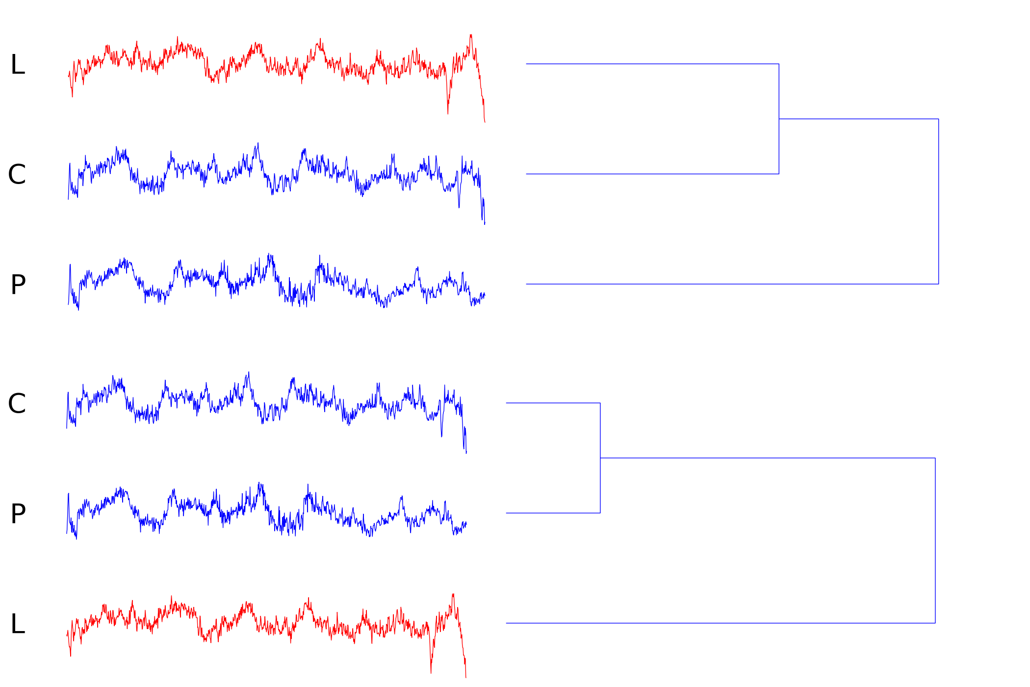
Index 194 (extraction failure/unknown scale)
Although all time series have been scaled to the same length to synchronize the sampling rate of both sensors it may happen, that the extraction of the signal from the data stream is imprecise. A close look at the dendrogram reveals that a slightly downscaled version of P fits a substantial region of C. GEM features scale and translation invariant subsequence matching in the time domain which enables us to find the correct mapping.
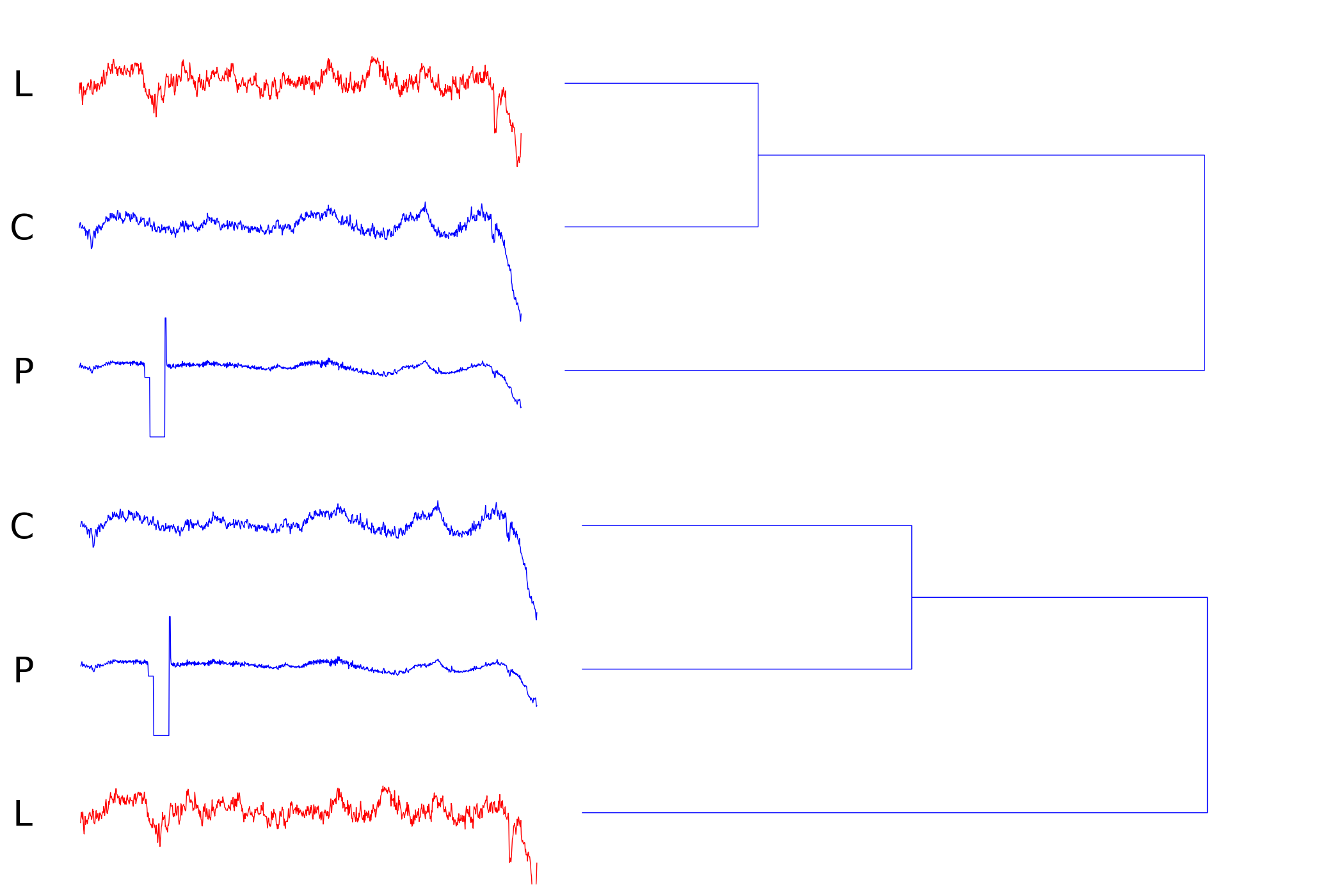
Index 255 (occlusion/sensor failure)
This example demonstrates how z-normalization can be harmful when sensor failure occurs. The amplitudes of the distorted time series (P) are significantly altered. GEM avoids this artifact since it does not use z-normalization and allows skips in the query or subject sequence.
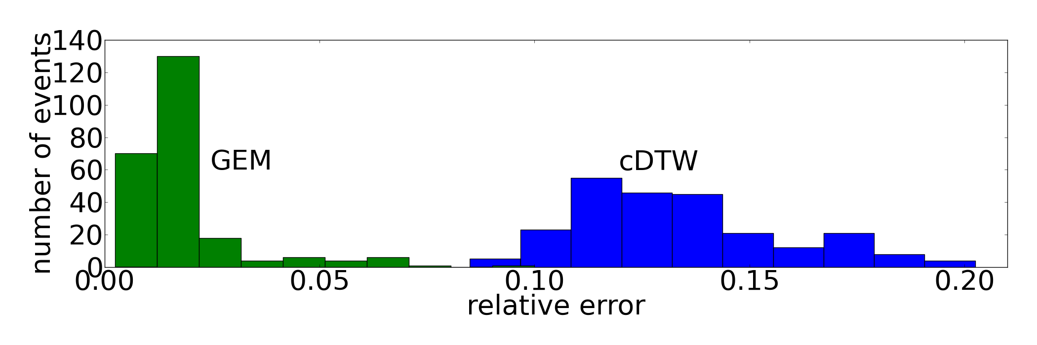
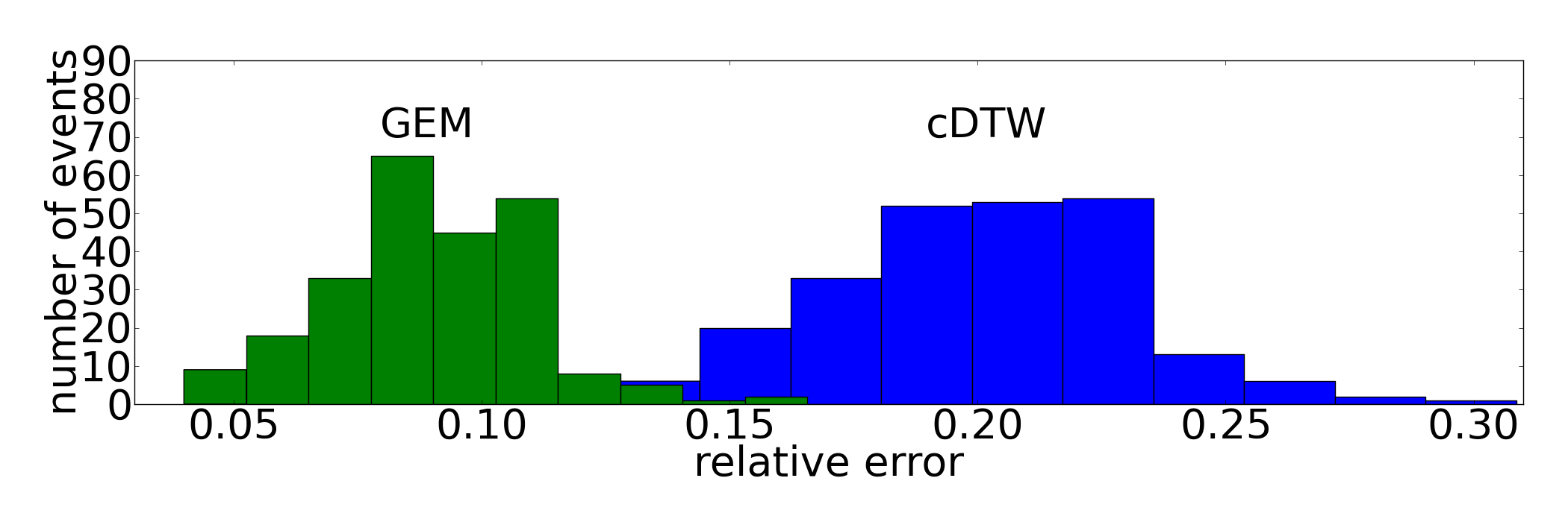
Metal and Fish resampled 1NN
Detailed information about all tested distance measures (GEM, (c)DTW, ED) the used splits and learned parameters can be found in the result folder (dn_M* and dn_39*). The histograms can be generated with ResultsMetall.py and ResultsFish.py.
Metal Protocol and Relative Error Rates
The metal dataset consists of 1000 pairs of thickness profile measurements of metal coils. Given a thickness measurement child^i we assign the corresponding time series parent^i for all i in {0,..., 999}. As a result, the dataset consists of 1000 classes with two members each. Since GEM and cDTW both depend on external parameters, we have to carry out parameter learning. Unfortunately, every stratified split of the dataset into a training and test set creates classes with exactly one member which renders parameter learning infeasible. Therefore, we separate a small subset for parameter learning beforehand and determine the error rates on the complementary set to avoid leakage. For our experiments we use the following protocol:
- (i) Shuffle the index set I:={0,...,999} with a random permutation pi to obtain pi(I):={pi(0),...,pi(999)}.
- (ii) Split pi(I) into four disjoint index subsets -- two pairs of parameter learning and holdout sets: (L_left, H_left) as well as (L_right, H_right) with |L_j| = 100 and |H_j| = 400 each.
- (iii) For each of the two pairs (L_j, H_j) do the following: Learn the parameters of the given distance measure on the indices L_j by picking the parameter that yields minimum classification error of a 1NN-classifier built with the parents. After picking the most promising parameter determine the 1NN-classification error on the complementary index set H_j in the same manner. Finally, one yields one error for each H_j. Go to (i) until finished.
The partition of the dataset is motivated by the following criteria: Parameters are learned on a small subset since this is the desired real-world setting. The parameter for cDTW is given by the relative window size of the Sakoe-Chiba Band and ranges from 0% to 20%. GEM's scaling parameters s_-, s_+ in S and the averaging coefficient alpha_1 in A are taken from the sets S={1,2} and A={2^{-p} | p in {1,...,8} }. Shuffling the indices during step (i) ensures variability of parameter learning scenarios. Additionally, the dataset is split into two pairs (L_j, H_j) to guarantee the same variability for the final error rate since H_j is substantially altered each run. Otherwise, we would end up with nearly identical holdout sets if we provided only one pair (L, H) for each iteration.
Fish/UCR Protocol and Relative Error Rates
The error rates for the members of the UCR repository are determined by the given protocol: Again, we consider a resampling strategy for our experiments to provide means and standard deviations. The fish dataset has been included into the UCR database and therefore a canonical split into a training and test set is provided. For further resampling we use the following protocol:
- (i) For the first iteration take the UCR split, otherwise accomplish a stratified random split of the dataset into a training and test set conserving the split and class ratios.
- (ii) Learn the parameters of the distance measures with Leave-One-Out-Cross-Validation (LOOCV) on the training set. Pick the parameter that minimizes the error rate.
- (iii) Build a 1NN-classifier with the training set and the optimal parameter. Determine the final error rate on the test set with this classifier. Return to (i) until finished.
UCR database resampled 1NN
The detailed classification rates for all tested distance measures (GEM, (c)DTW, ED) can be found here. This table can be generated with the given Python script. For even more details like the individual splits each iteration please have a look at the results folder.
| # | dataset | E_cdtw +/- Sigma | E_gem +/- Sigma |
|---|---|---|---|
| 0 | 50words | 0.2258 +/- 0.0161 | 0.2495 +/- 0.0202 |
| 1 | Adiac | 0.3743 +/- 0.0193 | 0.3004 +/- 0.0178 |
| 2 | Beef | 0.5387 +/- 0.0743 | 0.4860 +/- 0.0786 |
| 3 | CBF | 0.0080 +/- 0.0108 | 0.0003 +/- 0.0008 |
| 4 | Car | 0.2623 +/- 0.0463 | 0.1717 +/- 0.0434 |
| 5 | Chlorine | 0.3495 +/- 0.0104 | 0.3119 +/- 0.0110 |
| 6 | CinC_ECG | 0.0480 +/- 0.0256 | 0.0913 +/- 0.0306 |
| 7 | Coffee | 0.1470 +/- 0.0713 | 0.0283 +/- 0.0314 |
| 8 | Cricket_X | 0.1988 +/- 0.0199 | 0.2279 +/- 0.0227 |
| 9 | Cricket_Y | 0.1920 +/- 0.0214 | 0.2129 +/- 0.0183 |
| 10 | Cricket_Z | 0.1955 +/- 0.0170 | 0.2114 +/- 0.0204 |
| 11 | DiatomSize | 0.0224 +/- 0.0136 | 0.0361 +/- 0.0228 |
| 12 | ECG200 | 0.1282 +/- 0.0329 | 0.1264 +/- 0.0433 |
| 13 | ECG5Days | 0.1579 +/- 0.0518 | 0.1748 +/- 0.0459 |
| 14 | FaceAll | 0.0437 +/- 0.0219 | 0.0356 +/- 0.0260 |
| 15 | FaceFour | 0.1127 +/- 0.0444 | 0.1080 +/- 0.0610 |
| 16 | FacesUCR | 0.0793 +/- 0.0092 | 0.0605 +/- 0.0091 |
| 17 | Gun_Point | 0.0529 +/- 0.0262 | 0.0193 +/- 0.0113 |
| 18 | Haptics | 0.5771 +/- 0.0309 | 0.6113 +/- 0.0263 |
| 19 | InlineSkate | 0.5950 +/- 0.0216 | 0.5500 +/- 0.0227 |
| 20 | ItalyPower | 0.0583 +/- 0.0168 | 0.0533 +/- 0.0210 |
| 21 | Lighting2 | 0.1403 +/- 0.0361 | 0.1266 +/- 0.0433 |
| 22 | Lighting7 | 0.2455 +/- 0.0429 | 0.3504 +/- 0.0641 |
| 23 | MALLAT | 0.0474 +/- 0.0118 | 0.0573 +/- 0.0220 |
| 24 | MedicalImg | 0.2436 +/- 0.0118 | 0.2753 +/- 0.0186 |
| 25 | MoteStrain | 0.1478 +/- 0.0321 | 0.1385 +/- 0.0374 |
| 27 | OliveOil | 0.1268 +/- 0.0503 | 0.1199 +/- 0.0391 |
| 28 | SonyAIBO | 0.1212 +/- 0.0421 | 0.1364 +/- 0.0390 |
| 29 | SonyAIBO II | 0.1525 +/- 0.0256 | 0.1549 +/- 0.0240 |
| 30 | StarLightC. | running | running |
| 31 | SwedishLeaf | 0.1575 +/- 0.0150 | 0.1270 +/- 0.0143 |
| 32 | Symbols | 0.0722 +/- 0.0223 | 0.0386 +/- 0.0298 |
| 33 | Thorax1 | running | running |
| 34 | Thorax2 | running | running |
| 35 | Trace | 0.0004 +/- 0.0020 | 0.0034 +/- 0.0132 |
| 36 | TwoLeadECG | 0.1026 +/- 0.0626 | 0.0167 +/- 0.0249 |
| 37 | TwoPatterns | 0.0000 +/- 0.0001 | 0.0002 +/- 0.0003 |
| 38 | WordsSyno. | 0.2516 +/- 0.0161 | 0.2741 +/- 0.0188 |
| 39 | fish | 0.2003 +/- 0.0293 | 0.0895 +/- 0.0200 |
| 40 | plane | 0.0000 +/- 0.0000 | 0.0046 +/- 0.0067 |
| 41 | sy. control | 0.0108 +/- 0.0059 | 0.0367 +/- 0.0110 |
| 42 | UWGestureX | running | running |
| 43 | UWGestureY | running | running |
| 44 | UWGestureZ | running | running |
| 45 | wafer | 0.0051 +/- 0.0018 | 0.0048 +/- 0.0012 |
| 46 | yoga | 0.1465 +/- 0.0114 | 0.1463 +/- 0.0156 |
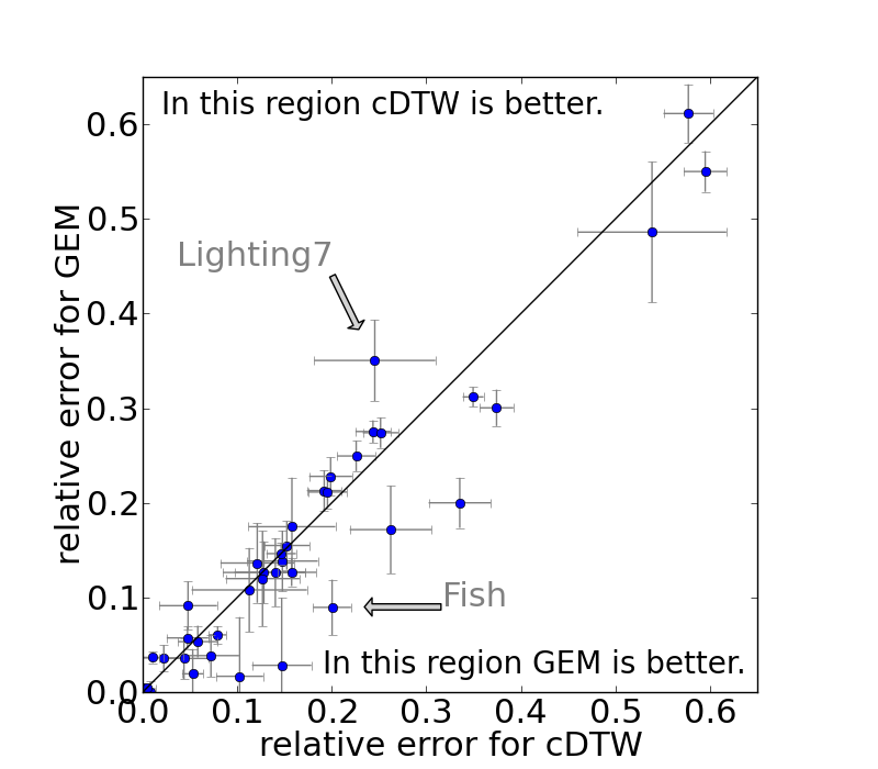
Visualized classification error
The averaged error rates and standard deviations (error bars) for constrained DTW and GEM on the individual datasets of the UCR repository are shown below.
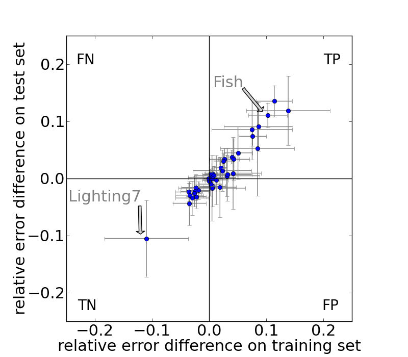
Prediction power (Texas sharpshooter plot)
The averaged differences of relative error rates and standard deviations (error bars) for constrained DTW and GEM (for both training and test set) on the individual datasets of the UCR repository are shown below.
Speedup Measurements
The makefile for the UCR Suite including the used compiler flags can be found here. The queries and subject of the ECG dataset are provided at the supplementary website of the UCR Suite. The queries and subject for the metal dataset can be generated with the given Python script.
The results for the ECG dataset are illustrated in the following figure:
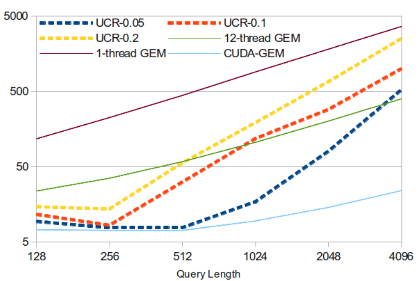 Figure: Performance in terms of execution time for the ECG dataset for the sequential (1 thread), OpenMP (12 threads), CUDA implementation of GEM in comparison to UCR-DTW with three different window settings (0.05, 0.1, 0.2). The x-axis represents the size of Q. S is fixed at size 20.1 million. The y-axis represents the execution time (in seconds), both using logarithmic scale.